12 Genome Environment Association
The lecture for this week can be found here.
All of the code presented in this weeks class comes modified from a former Marine Genomics student and recent UC Davis graduate, Camille Rumberger! Thank you Camille!
12.1 Download the data
For this week we are again using data from the wonderful Xuereb et al. 2018 paper here And consistes of a vcf file with 3966 Snps from 685 pacific sea cucumbers.
wget https://raw.githubusercontent.com/BayLab/MarineGenomicsData/main/week11_semester.tar.gz
tar -xzvf week11_semester.tar.gz
12.2 install a compiler for Unix/bash
Run this command below in the terminal. It’s necesary to install several R packages.
sudo apt install libgdal-dev12.3 install R packages
# devtools::install_github("bcm-uga/lfmm")
#
#
# # get packages
# install.packages(c('lfmm','psych','vegan','ggplot2','data.table','sdmpredictors','rgdal','raster'), dependencies = T)
# install.packages("BiocManager")
# BiocManager::install("LEA", force=T)

# call programs
library(lfmm)
library(psych)
library(vegan)
library(LEA)
library(data.table)
library(sdmpredictors)
library(leaflet)
library(ggplot2)
library(rgdal)
library(raster)
12.4 Get the Environmental Data
now we need to download the environmental data for our study. We’re just going to look at a few variables but there are many others that you could choose from here: https://www.bio-oracle.org/explore-data.php
Note that this step is rather time consuming, thus it’s best to download the data once and save it as an environment file, which you can upload each time you want to modify your script.
#load the environmental data and store it as objects that we can use later

environ <- load_layers(layercodes = c("BO_chlomean","BO_ph", "BO_salinity","BO_sstmax","BO_sstmean"))

#now put each layer into it's own object

chlomean<-load_layers("BO_chlomean")
ph<-load_layers("BO_ph")
salinity<-load_layers("BO_salinity")
sst_max<-load_layers("BO_sstmax")
sst_mean<-load_layers("BO_sstmean")
Now we’ll read in our metadata, which has lat and lon for each sample
meta<-read.csv("californicus_metadata.csv")

#make a new dataframe that just contains the lat and lon and label them "lat" and "long"
#notice that the original metafile mislabels lat and lon, oops!

sites<-cbind("lat" =  meta$LONG, "lon" = meta$LAT)

head(sites)
#>            lat     lon
#> [1,] -126.5646 50.5212
#> [2,] -126.5646 50.5212
#> [3,] -126.5646 50.5212
#> [4,] -126.5646 50.5212
#> [5,] -126.5646 50.5212
#> [6,] -126.5646 50.5212
12.5 Extract Site Specific Information from our Envirornmental Layers
The data we downloaded
sites_environ <- data.frame(Name=sites, extract(environ,sites))
head(sites_environ)
#>    Name.lat Name.lon BO_chlomean BO_ph BO_salinity BO_sstmax BO_sstmean
#> 1 -126.5646  50.5212        3.85 8.212      30.496    12.137        8.1
#> 2 -126.5646  50.5212        3.85 8.212      30.496    12.137        8.1
#> 3 -126.5646  50.5212        3.85 8.212      30.496    12.137        8.1
#> 4 -126.5646  50.5212        3.85 8.212      30.496    12.137        8.1
#> 5 -126.5646  50.5212        3.85 8.212      30.496    12.137        8.1
#> 6 -126.5646  50.5212        3.85 8.212      30.496    12.137        8.1
That produces for us a site specific environment file. We now need to convert this file into a format that we can save it as a matrix and export it as an environment file (i.e., in the format that the next step need it to be in which we do below)
#remove lat and lon and convert to matrix

sites_environ_matrix<-as.matrix(sites_environ[,-c(1,2)])

#remove any Na's

sites_environ_matrix_nas<-na.omit(sites_environ_matrix)

#write the file to an env file

write.env(sites_environ_matrix_nas, "sites_environ_matrix.env")
#> [1] "sites_environ_matrix.env"
12.6 Make a Map of our environmental data
We now have enough information to make a pretty plot of one of our environmental parameters.
library(sdmpredictors)

#download a raster file for env variable that we want to look at

#what are are min amd max lat and lon

range(sites_environ$Name.lon)
#> [1] 48.40822 57.82796
#crop file to fit the area we want
ne.pacific<-extent(-140, -120, 40, 60)

sst_max.crop<-crop(sst_max, ne.pacific)


#make a nice color ramp and plot the map

my.colors = colorRampPalette(c("#5E85B8","#EDF0C0","#C13127"))
plot(sst_max.crop,col=my.colors(1000),axes=FALSE, box=FALSE)
title(cex.sub = 1.25, sub = "Maximum temperature at the sea surface (ºC)")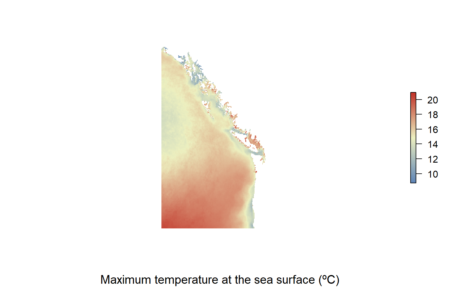
12.7 Load in genetic data
Now we need to load in our genetic data. We have data in a vcf file format and the first few steps will be to convert it to the format needed by the lfmm package.
loading the data in using these functions will output a lot to the console regarding the number of individuals (in this example 685) and loci (3699). It’s a good idea to look at these to make sure you have the number of individuals and loci that you expect. But it’s a but messy here so we’ve silenced that output.
#convert our vcf file to lfmm

vcf2lfmm('filtered_3699snps_californicus_685inds.recode.vcf', 'filtered_3699snps_californicus.lfmm')
#>
#>  - number of detected individuals:   685
#>  - number of detected loci:      3699
#>
#> For SNP info, please check ./filtered_3699snps_californicus_685inds.recode.vcfsnp.
#>
#> 0 line(s) were removed because these are not SNPs.
#> Please, check ./filtered_3699snps_californicus_685inds.recode.removed file, for more informations.
#>
#>
#>  - number of detected individuals:   685
#>  - number of detected loci:      3699
#> [1] "./filtered_3699snps_californicus_685inds.recode.lfmm"

sea_cuc_lfmm<-read.lfmm('filtered_3699snps_californicus_685inds.recode.lfmm')

#and convert to geno

lfmm2geno('filtered_3699snps_californicus_685inds.recode.lfmm', 'filtered_3699snps_californicus_685inds.recode.geno')
#>
#>  - number of detected individuals:   685
#>  - number of detected loci:      3699
#> [1] "filtered_3699snps_californicus_685inds.recode.geno"

#read in geno file

sea_cuc_geno<-read.geno('filtered_3699snps_californicus_685inds.recode.geno')
# create a snmf object

sea_cuc200.snmf <- snmf("filtered_3699snps_californicus_685.geno", K = 1:10, entropy=T, ploidy = 2, project = "new")
#> The project is saved into :
#>  filtered_3699snps_californicus_685.snmfProject
#>
#> To load the project, use:
#>  project = load.snmfProject("filtered_3699snps_californicus_685.snmfProject")
#>
#> To remove the project, use:
#>  remove.snmfProject("filtered_3699snps_californicus_685.snmfProject")
#>
#> [1] 220560942
#> [1] "*************************************"
#> [1] "*          create.dataset            *"
#> [1] "*************************************"
#>
#> ERROR: unable to open file C:\Users\SAPCaps\MarineGenomicsSemester\data\Week11_gea\filtered_3699snps_californicus_685.geno. Please, check that the name of the file you provided is correct.
#> Error in create.dataset(input.file, masked.file, s, percentage): internal error in trio library

project=load.snmfProject("filtered_3699snps_californicus_685.snmfProject")

#plot values of cross-entropy criteron of k
plot(sea_cuc200.snmf)
#> Error in h(simpleError(msg, call)): error in evaluating the argument 'x' in selecting a method for function 'plot': object 'sea_cuc200.snmf' not found
This plot tells us which value of K we should use when running the next analyses. We’re looking for a region where the cross-entropy is lowest and ideally it plateaus. We don’t get a plateau in our case but you can see our lowest value is at 3. So we would use a K of 3 in the next step.
However, for the purposes of time we’re going to do the next step with a k=1 and a rep=1.
# Genome scan for selection using environmental variables


sea_cuc_lfmm <- lfmm("filtered_3699snps_californicus_685inds.recode.lfmm", "sites_environ_matrix.env", K=1, rep=1, project = "new")
#> The project is saved into :
#>  filtered_3699snps_californicus_685inds.lfmmProject
#>
#> To load the project, use:
#>  project = load.lfmmProject("filtered_3699snps_californicus_685inds.lfmmProject")
#>
#> To remove the project, use:
#>  remove.lfmmProject("filtered_3699snps_californicus_685inds.lfmmProject")
#>
#> [1] "********************************"
#> [1] "* K = 1  repetition 1  d = 1   *"
#> [1] "********************************"
#> Summary of the options:
#>
#>         -n (number of individuals)      685
#>         -L (number of loci)             3699
#>         -K (number of latent factors)   1
#>         -o (output file)                filtered_3699snps_californicus_685inds.lfmm/K1/run1/filtered_3699snps_californicus_685inds.recode_r1
#>         -i (number of iterations)       10000
#>         -b (burnin)                     5000
#>         -s (seed random init)           1732907326
#>         -p (number of processes (CPU))  1
#>         -x (genotype file)              filtered_3699snps_californicus_685inds.recode.lfmm
#>         -v (variable file)              sites_environ_matrix.env
#>         -D (number of covariables)      5
#>         -d (the dth covariable)         1
#>
#> Read variable file:
#>      sites_environ_matrix.env        OK.
#>
#> Read genotype file:
#>      filtered_3699snps_californicus_685inds.recode.lfmm      OK.
#>
#> <<<<
#>   Analyse for variable 1
#>
#>      Start of the Gibbs Sampler algorithm.
#>
#>  [                                                                           ]
#>  [===========================================================================]
#>
#>      End of the Gibbs Sampler algorithm.
#>
#>  ED:2533818.105   DIC: 2533819.118
#>
#>  The statistics for the run are registered in:
#>          filtered_3699snps_californicus_685inds.lfmm/K1/run1/filtered_3699snps_californicus_685inds.recode_r1_s1.1.dic.
#>
#>  The zscores for variable 1 are registered in:
#>          filtered_3699snps_californicus_685inds.lfmm/K1/run1/filtered_3699snps_californicus_685inds.recode_r1_s1.1.zscore.
#>  The columns are: zscores, -log10(p-values), p-values.
#>
#>  -------------------------
#>  The execution for variable 1 worked without error.
#> >>>>
#>
#> The project is saved into :
#>  filtered_3699snps_californicus_685inds.lfmmProject
#>
#> To load the project, use:
#>  project = load.lfmmProject("filtered_3699snps_californicus_685inds.lfmmProject")
#>
#> To remove the project, use:
#>  remove.lfmmProject("filtered_3699snps_californicus_685inds.lfmmProject")
#>
#> [1] "********************************"
#> [1] "* K = 1  repetition 1  d = 2   *"
#> [1] "********************************"
#> Summary of the options:
#>
#>         -n (number of individuals)      685
#>         -L (number of loci)             3699
#>         -K (number of latent factors)   1
#>         -o (output file)                filtered_3699snps_californicus_685inds.lfmm/K1/run2/filtered_3699snps_californicus_685inds.recode_r2
#>         -i (number of iterations)       10000
#>         -b (burnin)                     5000
#>         -s (seed random init)           1732907326
#>         -p (number of processes (CPU))  1
#>         -x (genotype file)              filtered_3699snps_californicus_685inds.recode.lfmm
#>         -v (variable file)              sites_environ_matrix.env
#>         -D (number of covariables)      5
#>         -d (the dth covariable)         2
#>
#> Read variable file:
#>      sites_environ_matrix.env        OK.
#>
#> Read genotype file:
#>      filtered_3699snps_californicus_685inds.recode.lfmm      OK.
#>
#> <<<<
#>   Analyse for variable 2
#>
#>      Start of the Gibbs Sampler algorithm.
#>
#>  [                                                                           ]
#>  [===========================================================================]
#>
#>      End of the Gibbs Sampler algorithm.
#>
#>  ED:2533818.024   DIC: 2533819.058
#>
#>  The statistics for the run are registered in:
#>          filtered_3699snps_californicus_685inds.lfmm/K1/run2/filtered_3699snps_californicus_685inds.recode_r2_s2.1.dic.
#>
#>  The zscores for variable 2 are registered in:
#>          filtered_3699snps_californicus_685inds.lfmm/K1/run2/filtered_3699snps_californicus_685inds.recode_r2_s2.1.zscore.
#>  The columns are: zscores, -log10(p-values), p-values.
#>
#>  -------------------------
#>  The execution for variable 2 worked without error.
#> >>>>
#>
#> The project is saved into :
#>  filtered_3699snps_californicus_685inds.lfmmProject
#>
#> To load the project, use:
#>  project = load.lfmmProject("filtered_3699snps_californicus_685inds.lfmmProject")
#>
#> To remove the project, use:
#>  remove.lfmmProject("filtered_3699snps_californicus_685inds.lfmmProject")
#>
#> [1] "********************************"
#> [1] "* K = 1  repetition 1  d = 3   *"
#> [1] "********************************"
#> Summary of the options:
#>
#>         -n (number of individuals)      685
#>         -L (number of loci)             3699
#>         -K (number of latent factors)   1
#>         -o (output file)                filtered_3699snps_californicus_685inds.lfmm/K1/run3/filtered_3699snps_californicus_685inds.recode_r3
#>         -i (number of iterations)       10000
#>         -b (burnin)                     5000
#>         -s (seed random init)           1732907326
#>         -p (number of processes (CPU))  1
#>         -x (genotype file)              filtered_3699snps_californicus_685inds.recode.lfmm
#>         -v (variable file)              sites_environ_matrix.env
#>         -D (number of covariables)      5
#>         -d (the dth covariable)         3
#>
#> Read variable file:
#>      sites_environ_matrix.env        OK.
#>
#> Read genotype file:
#>      filtered_3699snps_californicus_685inds.recode.lfmm      OK.
#>
#> <<<<
#>   Analyse for variable 3
#>
#>      Start of the Gibbs Sampler algorithm.
#>
#>  [                                                                           ]
#>  [===========================================================================]
#>
#>      End of the Gibbs Sampler algorithm.
#>
#>  ED:2533818.091   DIC: 2533819.041
#>
#>  The statistics for the run are registered in:
#>          filtered_3699snps_californicus_685inds.lfmm/K1/run3/filtered_3699snps_californicus_685inds.recode_r3_s3.1.dic.
#>
#>  The zscores for variable 3 are registered in:
#>          filtered_3699snps_californicus_685inds.lfmm/K1/run3/filtered_3699snps_californicus_685inds.recode_r3_s3.1.zscore.
#>  The columns are: zscores, -log10(p-values), p-values.
#>
#>  -------------------------
#>  The execution for variable 3 worked without error.
#> >>>>
#>
#> The project is saved into :
#>  filtered_3699snps_californicus_685inds.lfmmProject
#>
#> To load the project, use:
#>  project = load.lfmmProject("filtered_3699snps_californicus_685inds.lfmmProject")
#>
#> To remove the project, use:
#>  remove.lfmmProject("filtered_3699snps_californicus_685inds.lfmmProject")
#>
#> [1] "********************************"
#> [1] "* K = 1  repetition 1  d = 4   *"
#> [1] "********************************"
#> Summary of the options:
#>
#>         -n (number of individuals)      685
#>         -L (number of loci)             3699
#>         -K (number of latent factors)   1
#>         -o (output file)                filtered_3699snps_californicus_685inds.lfmm/K1/run4/filtered_3699snps_californicus_685inds.recode_r4
#>         -i (number of iterations)       10000
#>         -b (burnin)                     5000
#>         -s (seed random init)           1732907326
#>         -p (number of processes (CPU))  1
#>         -x (genotype file)              filtered_3699snps_californicus_685inds.recode.lfmm
#>         -v (variable file)              sites_environ_matrix.env
#>         -D (number of covariables)      5
#>         -d (the dth covariable)         4
#>
#> Read variable file:
#>      sites_environ_matrix.env        OK.
#>
#> Read genotype file:
#>      filtered_3699snps_californicus_685inds.recode.lfmm      OK.
#>
#> <<<<
#>   Analyse for variable 4
#>
#>      Start of the Gibbs Sampler algorithm.
#>
#>  [                                                                           ]
#>  [===========================================================================]
#>
#>      End of the Gibbs Sampler algorithm.
#>
#>  ED:2533818.132   DIC: 2533819.128
#>
#>  The statistics for the run are registered in:
#>          filtered_3699snps_californicus_685inds.lfmm/K1/run4/filtered_3699snps_californicus_685inds.recode_r4_s4.1.dic.
#>
#>  The zscores for variable 4 are registered in:
#>          filtered_3699snps_californicus_685inds.lfmm/K1/run4/filtered_3699snps_californicus_685inds.recode_r4_s4.1.zscore.
#>  The columns are: zscores, -log10(p-values), p-values.
#>
#>  -------------------------
#>  The execution for variable 4 worked without error.
#> >>>>
#>
#> The project is saved into :
#>  filtered_3699snps_californicus_685inds.lfmmProject
#>
#> To load the project, use:
#>  project = load.lfmmProject("filtered_3699snps_californicus_685inds.lfmmProject")
#>
#> To remove the project, use:
#>  remove.lfmmProject("filtered_3699snps_californicus_685inds.lfmmProject")
#>
#> [1] "********************************"
#> [1] "* K = 1  repetition 1  d = 5   *"
#> [1] "********************************"
#> Summary of the options:
#>
#>         -n (number of individuals)      685
#>         -L (number of loci)             3699
#>         -K (number of latent factors)   1
#>         -o (output file)                filtered_3699snps_californicus_685inds.lfmm/K1/run5/filtered_3699snps_californicus_685inds.recode_r5
#>         -i (number of iterations)       10000
#>         -b (burnin)                     5000
#>         -s (seed random init)           1732907326
#>         -p (number of processes (CPU))  1
#>         -x (genotype file)              filtered_3699snps_californicus_685inds.recode.lfmm
#>         -v (variable file)              sites_environ_matrix.env
#>         -D (number of covariables)      5
#>         -d (the dth covariable)         5
#>
#> Read variable file:
#>      sites_environ_matrix.env        OK.
#>
#> Read genotype file:
#>      filtered_3699snps_californicus_685inds.recode.lfmm      OK.
#>
#> <<<<
#>   Analyse for variable 5
#>
#>      Start of the Gibbs Sampler algorithm.
#>
#>  [                                                                           ]
#>  [===========================================================================]
#>
#>      End of the Gibbs Sampler algorithm.
#>
#>  ED:2533818.015   DIC: 2533819.004
#>
#>  The statistics for the run are registered in:
#>          filtered_3699snps_californicus_685inds.lfmm/K1/run5/filtered_3699snps_californicus_685inds.recode_r5_s5.1.dic.
#>
#>  The zscores for variable 5 are registered in:
#>          filtered_3699snps_californicus_685inds.lfmm/K1/run5/filtered_3699snps_californicus_685inds.recode_r5_s5.1.zscore.
#>  The columns are: zscores, -log10(p-values), p-values.
#>
#>  -------------------------
#>  The execution for variable 5 worked without error.
#> >>>>
#>
#> The project is saved into :
#>  filtered_3699snps_californicus_685inds.lfmmProject
#>
#> To load the project, use:
#>  project = load.lfmmProject("filtered_3699snps_californicus_685inds.lfmmProject")
#>
#> To remove the project, use:
#>  remove.lfmmProject("filtered_3699snps_californicus_685inds.lfmmProject")

# load project
project = load.lfmmProject("filtered_3699snps_californicus_685inds.lfmmProject")
Now we can check and see which of our environmental variables is association with genomic variation
#get the z scores from each run
zs<-lapply(1:5, function(x) z.scores(sea_cuc_lfmm, d=x))
# compute the genomic inflation factor lambda
lambdas<-lapply(1:5, function(x) median(zs[[x]]^2/qchisq(0.5, df=1)))
#then compute adjusted p-values
adj.p.vals<-lapply(1:5, function(x) pchisq(zs[[x]]^2/lambdas[[x]], df=1, lower=F))
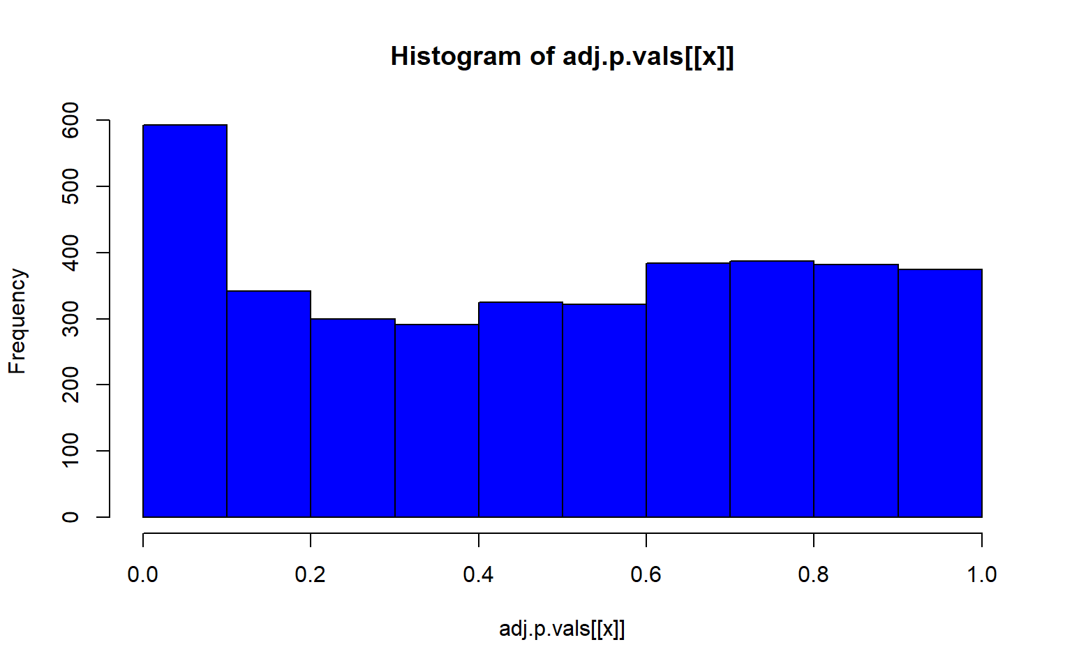
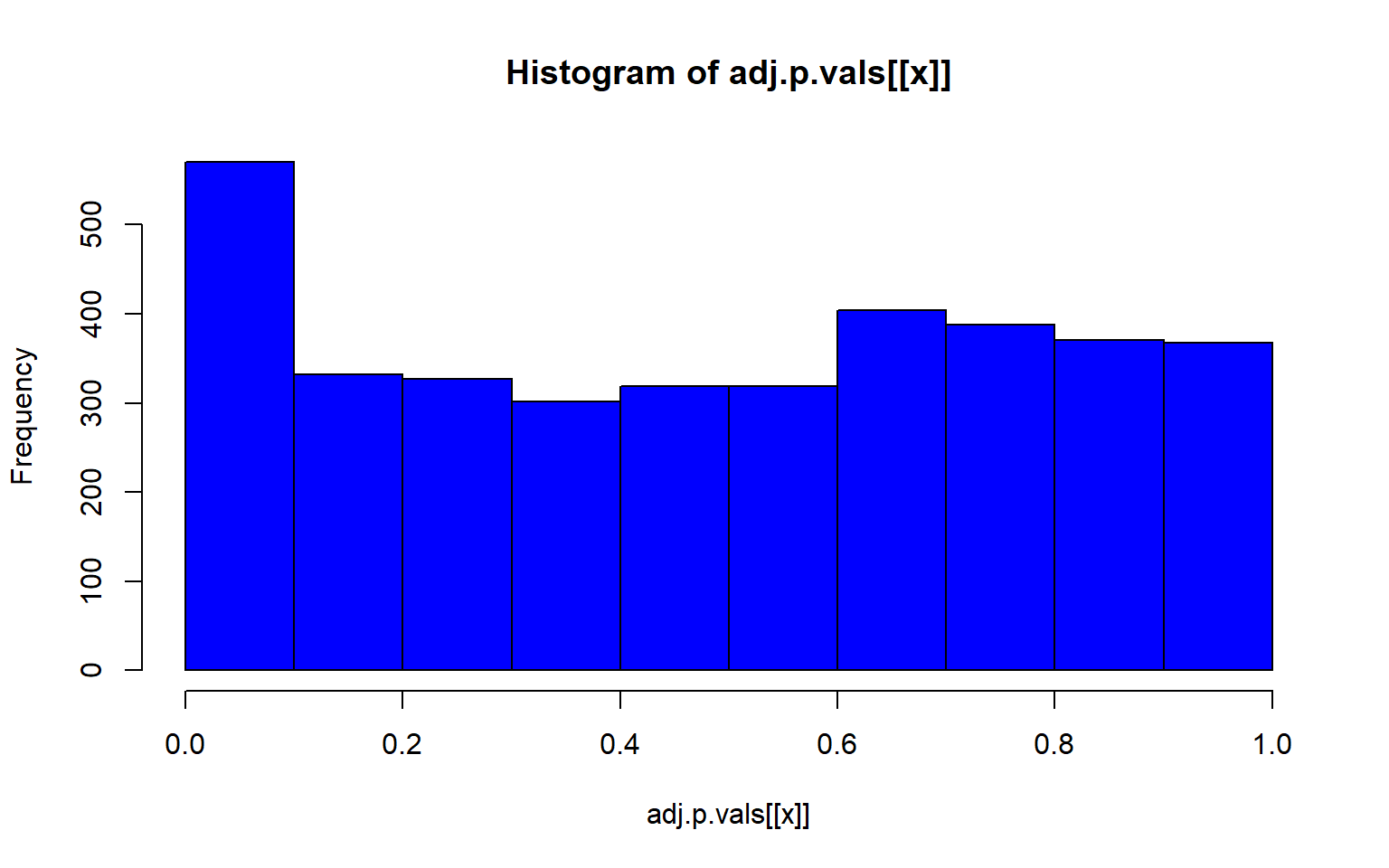
#then plot that p-value
lapply(1:5, function(x) hist(adj.p.vals[[x]], col="blue"))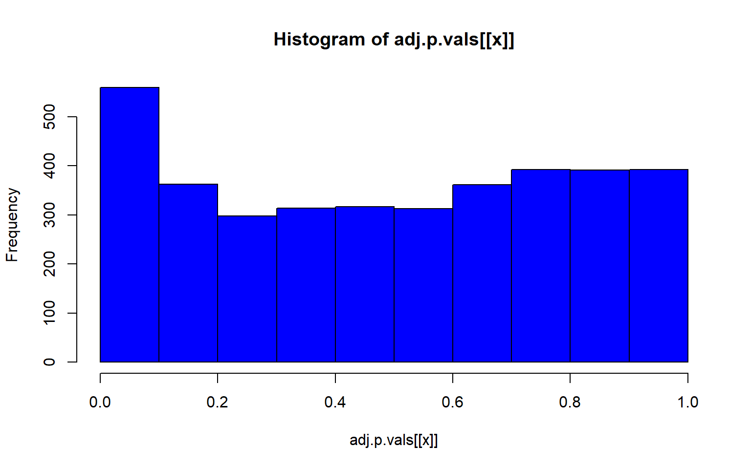
#> [[1]]
#> $breaks
#> [1] 0.0 0.1 0.2 0.3 0.4 0.5 0.6 0.7 0.8 0.9 1.0
#>
#> $counts
#> [1] 559 362 298 314 317 313 361 392 391 392
#>
#> $density
#> [1] 1.5112192 0.9786429 0.8056231 0.8488781 0.8569884 0.8461746 0.9759394 1.0597459 1.0570424 1.0597459
#>
#> $mids
#> [1] 0.05 0.15 0.25 0.35 0.45 0.55 0.65 0.75 0.85 0.95
#>
#> $xname
#> [1] "adj.p.vals[[x]]"
#>
#> $equidist
#> [1] TRUE
#>
#> attr(,"class")
#> [1] "histogram"
#>
#> [[2]]
#> $breaks
#> [1] 0.0 0.1 0.2 0.3 0.4 0.5 0.6 0.7 0.8 0.9 1.0
#>
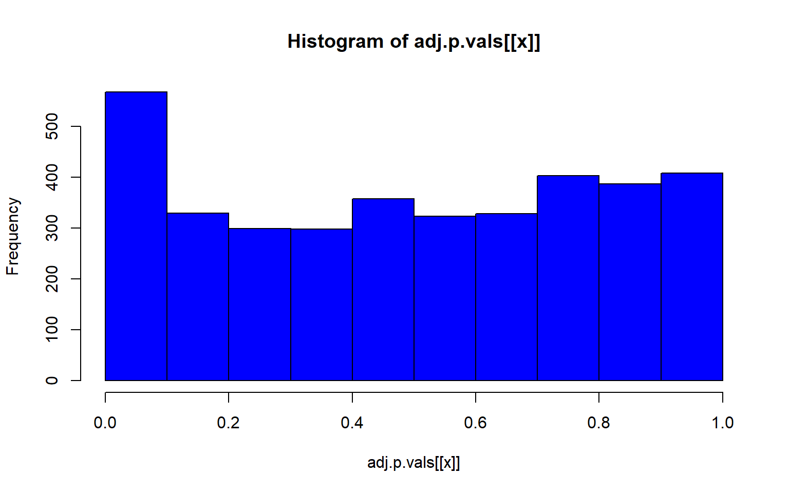
#> $counts
#> [1] 567 329 299 298 357 323 328 403 387 408
#>
#> $density
#> [1] 1.5328467 0.8894296 0.8083266 0.8056231 0.9651257 0.8732090 0.8867261 1.0894836 1.0462287 1.1030008
#>
#> $mids
#> [1] 0.05 0.15 0.25 0.35 0.45 0.55 0.65 0.75 0.85 0.95
#>
#> $xname
#> [1] "adj.p.vals[[x]]"
#>
#> $equidist
#> [1] TRUE
#>
#> attr(,"class")
#> [1] "histogram"
#>
#> [[3]]
#> $breaks
#> [1] 0.0 0.1 0.2 0.3 0.4 0.5 0.6 0.7 0.8 0.9 1.0
#>
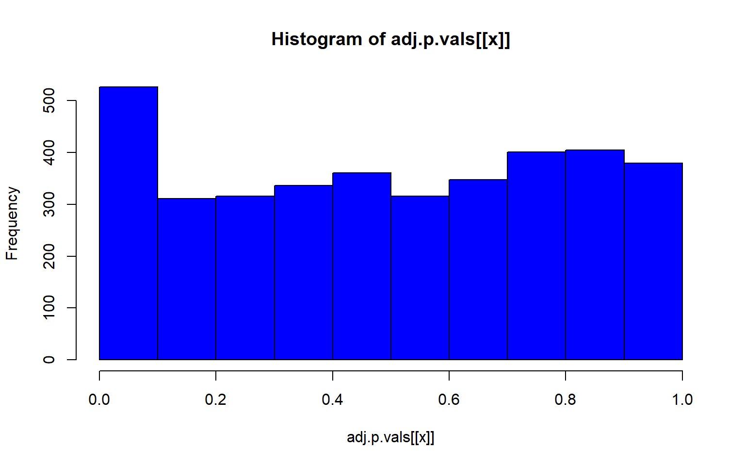
#> $counts
#> [1] 526 311 316 336 361 316 348 401 405 379
#>
#> $density
#> [1] 1.4220059 0.8407678 0.8542849 0.9083536 0.9759394 0.8542849 0.9407948 1.0840768 1.0948905 1.0246012
#>
#> $mids
#> [1] 0.05 0.15 0.25 0.35 0.45 0.55 0.65 0.75 0.85 0.95
#>
#> $xname
#> [1] "adj.p.vals[[x]]"
#>
#> $equidist
#> [1] TRUE
#>
#> attr(,"class")
#> [1] "histogram"
#>
#> [[4]]
#> $breaks
#> [1] 0.0 0.1 0.2 0.3 0.4 0.5 0.6 0.7 0.8 0.9 1.0
#>
#> $counts
#> [1] 592 342 300 291 325 322 384 387 382 374
#>
#> $density
#> [1] 1.6004325 0.9245742 0.8110300 0.7866991 0.8786158 0.8705055 1.0381184 1.0462287 1.0327115 1.0110841
#>
#> $mids
#> [1] 0.05 0.15 0.25 0.35 0.45 0.55 0.65 0.75 0.85 0.95
#>
#> $xname
#> [1] "adj.p.vals[[x]]"
#>
#> $equidist
#> [1] TRUE
#>
#> attr(,"class")
#> [1] "histogram"
#>
#> [[5]]
#> $breaks
#> [1] 0.0 0.1 0.2 0.3 0.4 0.5 0.6 0.7 0.8 0.9 1.0
#>
#> $counts
#> [1] 570 332 327 302 319 319 404 388 371 367
#>
#> $density
#> [1] 1.5409570 0.8975399 0.8840227 0.8164369 0.8623952 0.8623952 1.0921871 1.0489321 1.0029738 0.9921600
#>
#> $mids
#> [1] 0.05 0.15 0.25 0.35 0.45 0.55 0.65 0.75 0.85 0.95
#>
#> $xname
#> [1] "adj.p.vals[[x]]"
#>
#> $equidist
#> [1] TRUE
#>
#> attr(,"class")
#> [1] "histogram"
# control of false discoveries
# to correct for multiple testing, we can apply the Benjamini-Hochberg algorithm
# L is number of loci
L=3699
#fdr level q
q = 0.1
w = which(sort(adj.p.val1) < q * (1:L)/L)
# candidates are then
candidates.1 = order(adj.p.val1)[w]
length(candidates.1)
#> [1] 86
#this is for our first variable Mean Chlorphyl
12.8 Exercises
- Pick your favorite environmental variable from the bio-oracle website. For marine variables you can use the command
list_layers(c("Bio-ORACLE","MARSPEC"))$layer_codeto view the different Bio-Oracle and MARSPEC environmental layers. For Terrestrial layers use:list_layers("WorldClim")$layer_codeThen download the layer you choose and store it as an object withload_layers()Now decide which region you want to plot. If you’re interested in getting most of California you can use these coords with the function extent(-125, -115, 30, 40), and then use that to crop your environmental layers and make a plot similiar to the one we made in class.
Solution
library(sdmpredictors)

#get env data
precip_seasonality<-load_layers("WC_bio15")

precip_wettest<-load_layers("WC_bio13")

#make range to crop for california
cali<-extent(-130, -116, 30, 40)

#crop it

precip_w.crop<-crop(precip_wettest, cali)


#plot it

my.colors = colorRampPalette(c("#5E85B8","#EDF0C0","#C13127"))
plot(precip_w.crop,col=my.colors(1000),axes=FALSE, box=FALSE)
  title(cex.sub = 1.25, sub = "Precipitation of the Wettest Month")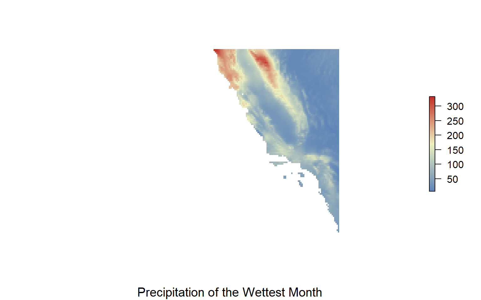
- Use the script for determining the number of candidates for the first environmental variable, find the number of candidates for the other four variables. Are these the same or different SNPs? (hint use merge() or intersect() to find out if the lists of candidates overlap)
Solution
#We'll use this script below

#for variable 2 (PH)
# L is number of loci
L=3699
#fdr level q
q = 0.1
w = which(sort(adj.p.val2) < q * (1:L)/L)
# candidates are then
candidates.2 = order(adj.p.val2)[w]

length(candidates.2)
#> [1] 59


#variable 3
w = which(sort(adj.p.val3) < q * (1:L)/L)
# candidates are then
candidates.3 = order(adj.p.val3)[w]

length(candidates.3)
#> [1] 78

#variable 4

w = which(sort(adj.p.val4) < q * (1:L)/L)
# candidates are then
candidates.4 = order(adj.p.val4)[w]

length(candidates.4)
#> [1] 58


#variable 5

w = which(sort(adj.p.val5) < q * (1:L)/L)
# candidates are then
candidates.5 = order(adj.p.val5)[w]

length(candidates.5)
#> [1] 114