8 Week 7 For loops and the apply family of functions
A few useful commands: function(), is.na, which, var, length, for(){ }, points, print, paste, plot, unique, sample
for loops: In many languages, the best way to repeat a calculation is to use a for-loop: For example, we could square each number 1 to 10
squares = rep(NA, 10) # use rep to create a vector length 10 of NAs to store the result
for (i in 1:10) { # for loop
  squares[i] = i^2
}
squares
#>  [1]   1   4   9  16  25  36  49  64  81 100
An alternative to for-loops in R is using the ‘apply’ family, while for-loops apply a function to one item at a time and then go on to the next one, “apply” applies functions to every item at once ## apply family ### sapply There are several apply functions that vary in the output the return and vary somewhat in the input they require. We’ll go over sapply “simplifying” apply which returns a vector, first.
#?sapply
# syntax: sapply(X = object_to_repeat_over, FUN = function_to_repeat)
# simple example of sapply over a vector
# we can use an in-line function definition
sapply(1:10, function(x)  x^2)
#>  [1]   1   4   9  16  25  36  49  64  81 100
# equivalently, we can define our own functions separately for sapply
# e.g. a function that calculates the area of a circle radius r, pi*r^2
areaCircle = function(r){
  return(pi * r^2)
}
sapply(1:10, areaCircle)
#>  [1]   3.141593  12.566371  28.274334  50.265482  78.539816 113.097336 153.938040 201.061930 254.469005 314.159265
# in R, we can also just use short-hand for simple vector calculations:
pi*(1:10)^2
#>  [1]   3.141593  12.566371  28.274334  50.265482  78.539816 113.097336 153.938040 201.061930 254.469005 314.159265
# but unlike the short-hand, sapply can also iterate over elements in a list
listy = list(a = TRUE, b = c("a", "b", "c"), c = 10:100)
str(listy) # look at the structure of 'listy'
#> List of 3
#>  $ a: logi TRUE
#>  $ b: chr [1:3] "a" "b" "c"
#>  $ c: int [1:91] 10 11 12 13 14 15 16 17 18 19 ...
length(listy) # look at the length of 'listy'
#> [1] 3
# use sapply to return a vector for length of each object within the list
sapply(listy, FUN = length)
#>  a  b  c
#>  1  3 91
You can also use sapply to create plots! For example, use sapply to plot these 4 dataframes at once:
df1 = data.frame(x1 = 1:10, y1 = 1:10)
df2 = data.frame(x2 = 1:10, y2 = -1:-10)
df3 = data.frame(x3 = 1:10, y3 = 10:1)
df4 = data.frame(x4 = 1:10, y4 = 1:10)
my_list = list(df1, df2, df3, df4) # put 4 data frames together in a list
par(mfrow = c(2,2)) # set up frame for 4 plots
sapply(my_list, plot) # plot my_list with sapply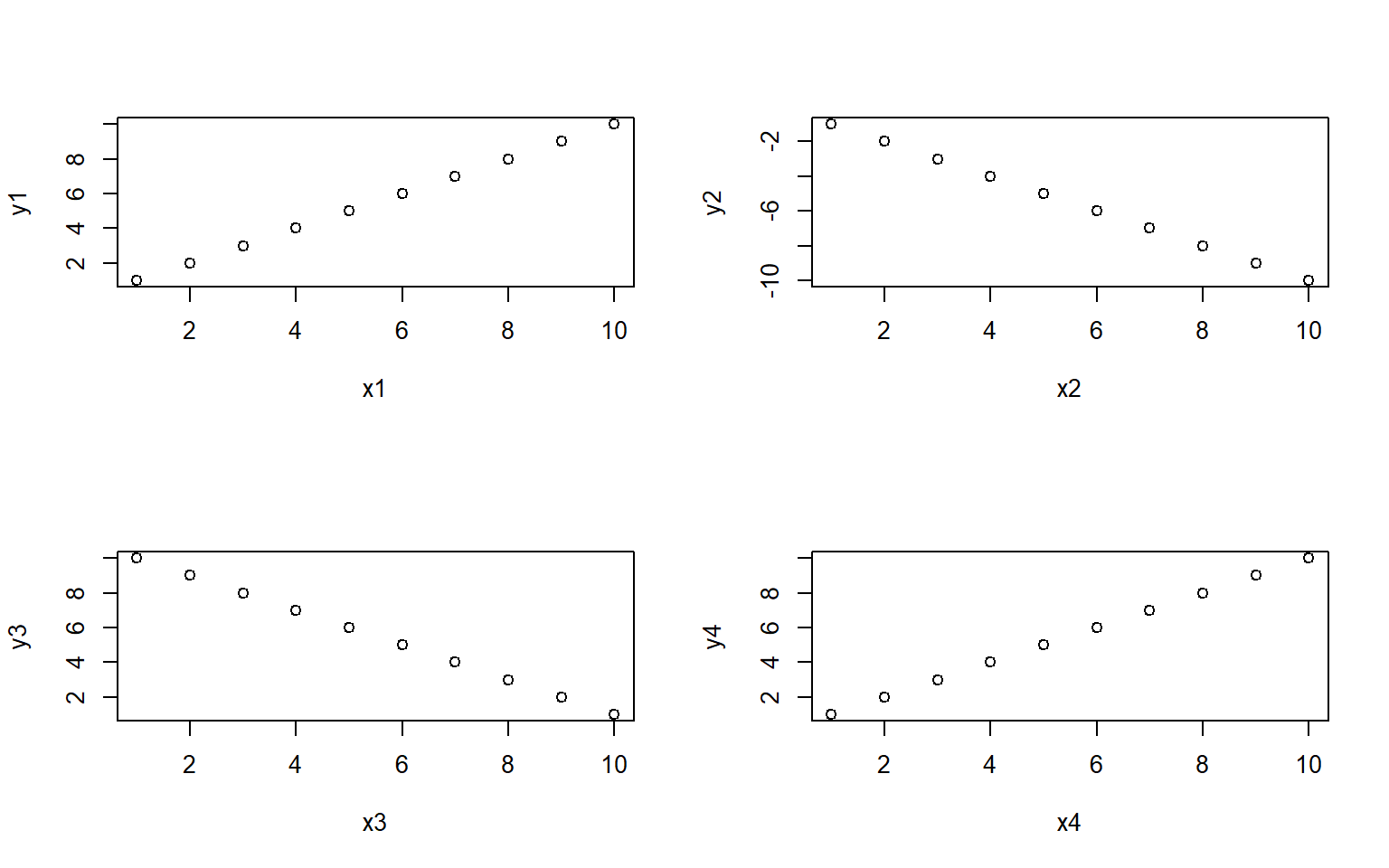
#> [[1]]
#> NULL
#>
#> [[2]]
#> NULL
#>
#> [[3]]
#> NULL
#>
#> [[4]]
#> NULL
8.0.1 apply
The apply function is highly useful for applying a function to rows or columns of a dataframe or matrix.
Example syntax for the dataframe or matrix X:
apply(X = over this object, MARGIN 1 for rows or 2 for columns,FUN = apply this function)
You can also use apply on a dataframe we worked with earlier the states data to plot each column against Population
#load in the data
data(state)
states = as.data.frame(state.x77) # convert data to a familiar format - data frame
str(states) # let's take a look at the dataframe
#> 'data.frame':    50 obs. of  8 variables:
#>  $ Population: num  3615 365 2212 2110 21198 ...
#>  $ Income    : num  3624 6315 4530 3378 5114 ...
#>  $ Illiteracy: num  2.1 1.5 1.8 1.9 1.1 0.7 1.1 0.9 1.3 2 ...
#>  $ Life Exp  : num  69 69.3 70.5 70.7 71.7 ...
#>  $ Murder    : num  15.1 11.3 7.8 10.1 10.3 6.8 3.1 6.2 10.7 13.9 ...
#>  $ HS Grad   : num  41.3 66.7 58.1 39.9 62.6 63.9 56 54.6 52.6 40.6 ...
#>  $ Frost     : num  20 152 15 65 20 166 139 103 11 60 ...
#>  $ Area      : num  50708 566432 113417 51945 156361 ...
# calculate the mean for each column
apply(states, 2, mean)
#> Population     Income Illiteracy   Life Exp     Murder    HS Grad      Frost       Area
#>  4246.4200  4435.8000     1.1700    70.8786     7.3780    53.1080   104.4600 70735.8800
# note you could get this with colMeans() or summary(), along with the min and max and other values, but there may be instances where you only want the mean
# you could also plot each column against Population in ggplotapply(states, 2, FUN = function(i) ggplot(states, aes(x=Population, y = i))+geom_point()+geom_smooth(method="lm")+theme_classic())
#> $Population
#> `geom_smooth()` using formula 'y ~ x'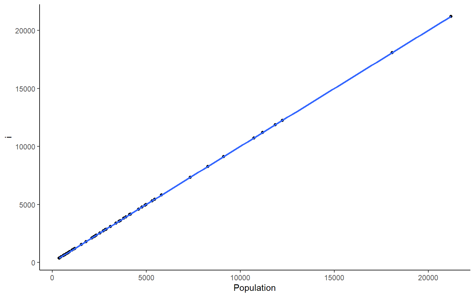
#>
#> $Income
#> `geom_smooth()` using formula 'y ~ x'
#>
#> $Illiteracy
#> `geom_smooth()` using formula 'y ~ x'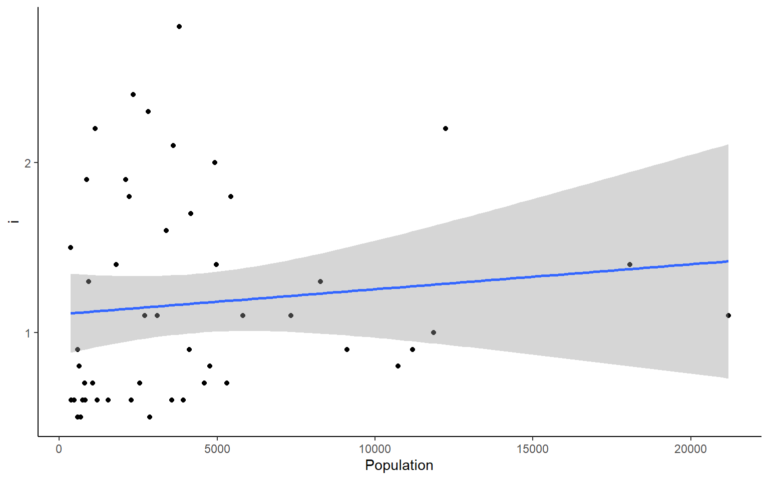
#>
#> $`Life Exp`
#> `geom_smooth()` using formula 'y ~ x'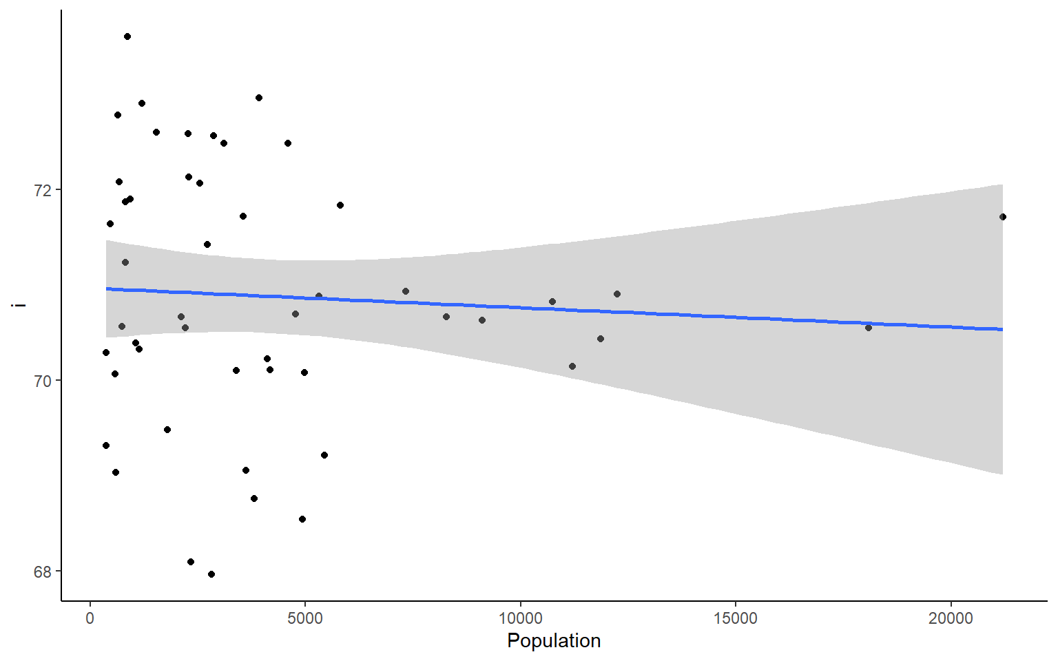
#>
#> $Murder
#> `geom_smooth()` using formula 'y ~ x'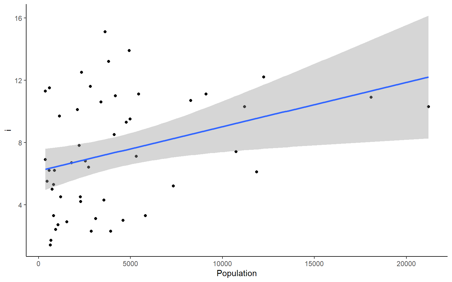
#>
#> $`HS Grad`
#> `geom_smooth()` using formula 'y ~ x'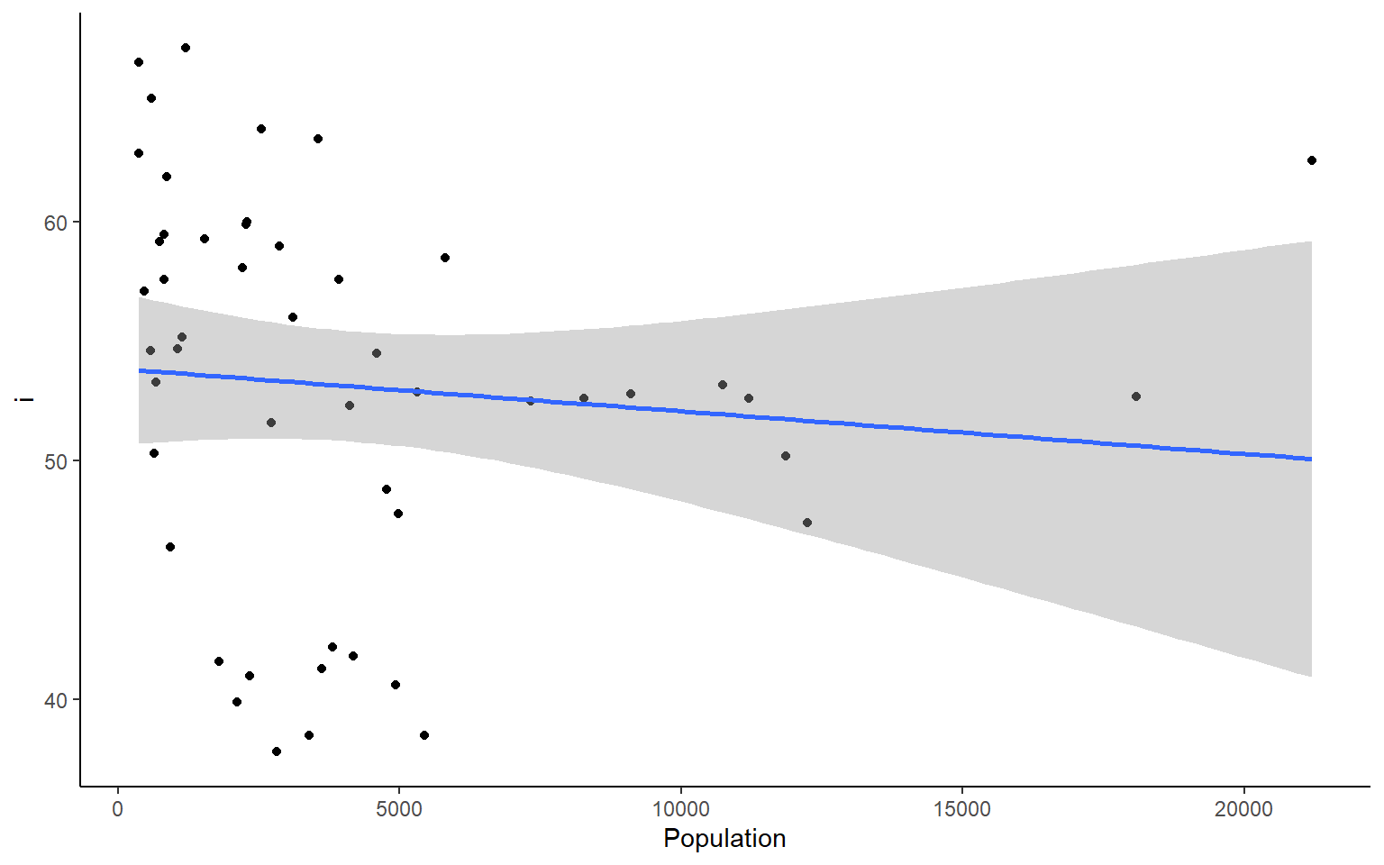
#>
#> $Frost
#> `geom_smooth()` using formula 'y ~ x'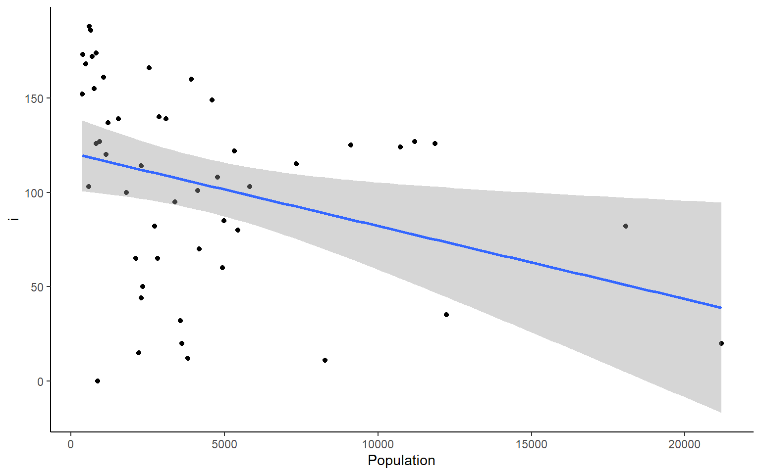
#>
#> $Area
#> `geom_smooth()` using formula 'y ~ x'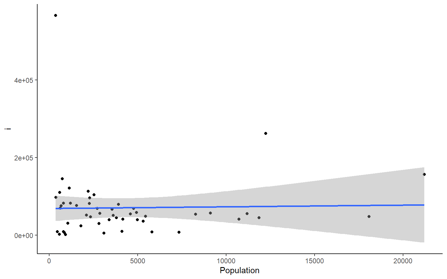 We can do the same things across all rows. But if you want to plot all the rows as we did the columns above, I suggest you do that with a smaller dataset than the states dataframe.
#calculate the sum across each row in states
apply(states, 1, sum)
#>        Alabama         Alaska        Arizona       Arkansas     California       Colorado    Connecticut       Delaware
#>       58094.55      573412.81      120312.25       57620.56      182838.71      111500.46       13581.68        7604.76
#>        Florida        Georgia         Hawaii          Idaho       Illinois        Indiana           Iowa         Kansas
#>       67328.26       67280.04       12399.60       87872.27       72312.94       46121.58       63704.36       88987.58
#>       Kentucky      Louisiana          Maine       Maryland  Massachusetts       Michigan      Minnesota    Mississippi
#>       46964.80       52419.96       35961.49       19544.92       18632.73       70939.43       88178.46       52908.99
#>       Missouri        Montana       Nebraska         Nevada  New Hampshire     New Jersey     New Mexico       New York
#>       78253.59      150970.36       82809.40      115962.23       14426.83       20335.73      126414.42       71027.55
#> North Carolina   North Dakota           Ohio       Oklahoma         Oregon   Pennsylvania   Rhode Island South Carolina
#>       58314.61       75308.28       56527.22       75692.52      103308.93       61528.73        6787.00       36860.66
#>   South Dakota      Tennessee          Texas           Utah        Vermont       Virginia     Washington  West Virginia
#>       81102.58       49516.61      278726.70       87603.30       13948.84       49675.78       75165.12       29705.18
#>      Wisconsin        Wyoming
#>       63800.68      102458.69
8.0.2 lapply – “list” apply
We’ll just show a quick example of lapply. It works in the same way as sapply, but returns a list instead of a vector.
lapply(1:10, function(x)  x^2) # lapply returns list
#> [[1]]
#> [1] 1
#>
#> [[2]]
#> [1] 4
#>
#> [[3]]
#> [1] 9
#>
#> [[4]]
#> [1] 16
#>
#> [[5]]
#> [1] 25
#>
#> [[6]]
#> [1] 36
#>
#> [[7]]
#> [1] 49
#>
#> [[8]]
#> [1] 64
#>
#> [[9]]
#> [1] 81
#>
#> [[10]]
#> [1] 100
sapply(1:10, function(x)  x^2, simplify = FALSE) # same as an lapply
#> [[1]]
#> [1] 1
#>
#> [[2]]
#> [1] 4
#>
#> [[3]]
#> [1] 9
#>
#> [[4]]
#> [1] 16
#>
#> [[5]]
#> [1] 25
#>
#> [[6]]
#> [1] 36
#>
#> [[7]]
#> [1] 49
#>
#> [[8]]
#> [1] 64
#>
#> [[9]]
#> [1] 81
#>
#> [[10]]
#> [1] 100
sapply(1:10, function(x)  x^2) # default is simplify = TRUE which retuns a vector
#>  [1]   1   4   9  16  25  36  49  64  81 100
8.0.3 tapply - “per Type” apply
The tapply function is one of my favorites because it is a really great way to sumarize data that has multiple categorical variables that can be
# load state data again, you can skip this if you already have it loaded
data(state)
states = as.data.frame(state.x77) # convert data to a familiar format - data frame
str(states) # let's take a look at the dataframe
#> 'data.frame':    50 obs. of  8 variables:
#>  $ Population: num  3615 365 2212 2110 21198 ...
#>  $ Income    : num  3624 6315 4530 3378 5114 ...
#>  $ Illiteracy: num  2.1 1.5 1.8 1.9 1.1 0.7 1.1 0.9 1.3 2 ...
#>  $ Life Exp  : num  69 69.3 70.5 70.7 71.7 ...
#>  $ Murder    : num  15.1 11.3 7.8 10.1 10.3 6.8 3.1 6.2 10.7 13.9 ...
#>  $ HS Grad   : num  41.3 66.7 58.1 39.9 62.6 63.9 56 54.6 52.6 40.6 ...
#>  $ Frost     : num  20 152 15 65 20 166 139 103 11 60 ...
#>  $ Area      : num  50708 566432 113417 51945 156361 ...
# example syntax --- tapply(variable of interest, grouping variable, function)
# for each US region in our dataset, finds the mean of Frost for states in that region
tapply(states$Frost, state.region, mean) # state.region contains the region information for each state
#>     Northeast         South North Central          West
#>      132.7778       64.6250      138.8333      102.1538
# you can nest apply statements! Let's find the region average for all the variables in the states dataset
apply(states,
      2, # apply over columns of my_states
      function(x) tapply(x, state.region, mean)) # each column = variable of interest for tapply
#>               Population   Income Illiteracy Life Exp    Murder  HS Grad    Frost      Area
#> Northeast       5495.111 4570.222   1.000000 71.26444  4.722222 53.96667 132.7778  18141.00
#> South           4208.125 4011.938   1.737500 69.70625 10.581250 44.34375  64.6250  54605.12
#> North Central   4803.000 4611.083   0.700000 71.76667  5.275000 54.51667 138.8333  62652.00
#> West            2915.308 4702.615   1.023077 71.23462  7.215385 62.00000 102.1538 134463.00
8.1 Exercise 2.3 apply and tapply
Exercise 2.3
A few useful commands: function(){ }, apply(), tapply(), hist(), dim(), prod(), sd() 1. what is the average population, income, and area of all 50 states ins the
statesdataset
Solution
# load state data
#?state
data(state)
# this data is stored in a slightly different way than other datasets we've used so far
states = as.data.frame(state.x77) # run this line of code to avoid later confusion
apply(states,2,mean)
#> Population     Income Illiteracy   Life Exp     Murder    HS Grad      Frost       Area
#>  4246.4200  4435.8000     1.1700    70.8786     7.3780    53.1080   104.4600 70735.8800
#or an alternative that will get you only the columns requested
colMeans(states[,c("Population", "Income", "Area")])
#> Population     Income       Area
#>    4246.42    4435.80   70735.88
- what is the average area of the states from different regions of the country? Hint: use the object state.region in your environment
Solution
tapply(states$Area, state.region, mean)
#>     Northeast         South North Central          West
#>      18141.00      54605.12      62652.00     134463.00
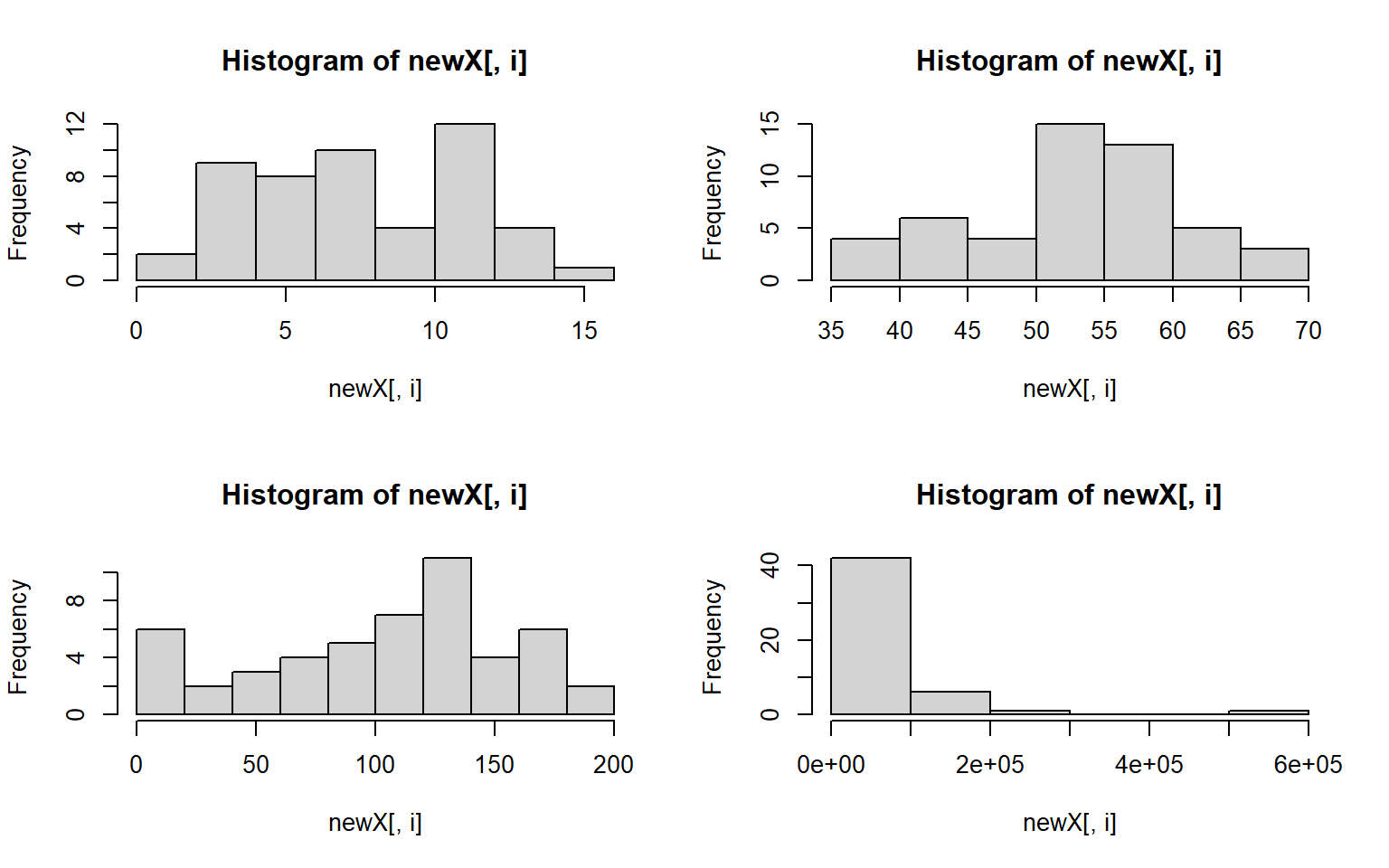
- Plot a histogram for each column in the states data (Population, Income, Illiteracy etc.)
Solution
#how many columns do we have?
dim(states)
#> [1] 50  8
par(mfrow = c(2,2)) # make your plot window show 2 rows and 2 columns at once
apply(states, 2, hist)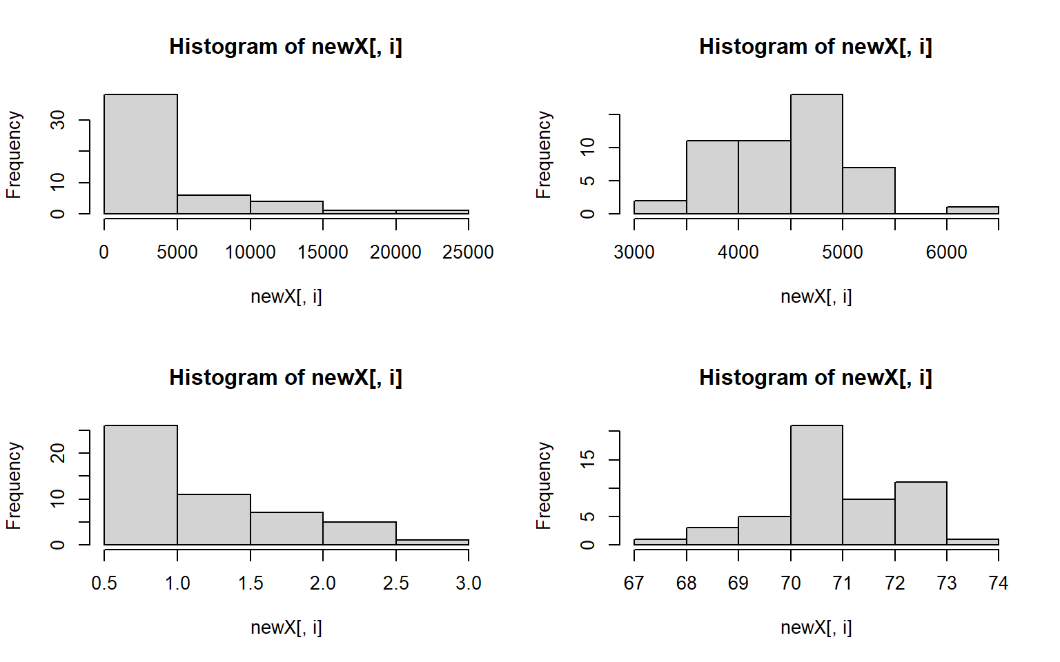
#> $Population
#> $breaks
#> [1]     0  5000 10000 15000 20000 25000
#>
#> $counts
#> [1] 38  6  4  1  1
#>
#> $density
#> [1] 0.000152 0.000024 0.000016 0.000004 0.000004
#>
#> $mids
#> [1]  2500  7500 12500 17500 22500
#>
#> $xname
#> [1] "newX[, i]"
#>
#> $equidist
#> [1] TRUE
#>
#> attr(,"class")
#> [1] "histogram"
#>
#> $Income
#> $breaks
#> [1] 3000 3500 4000 4500 5000 5500 6000 6500
#>
#> $counts
#> [1]  2 11 11 18  7  0  1
#>
#> $density
#> [1] 0.00008 0.00044 0.00044 0.00072 0.00028 0.00000 0.00004
#>
#> $mids
#> [1] 3250 3750 4250 4750 5250 5750 6250
#>
#> $xname
#> [1] "newX[, i]"
#>
#> $equidist
#> [1] TRUE
#>
#> attr(,"class")
#> [1] "histogram"
#>
#> $Illiteracy
#> $breaks
#> [1] 0.5 1.0 1.5 2.0 2.5 3.0
#>
#> $counts
#> [1] 26 11  7  5  1
#>
#> $density
#> [1] 1.04 0.44 0.28 0.20 0.04
#>
#> $mids
#> [1] 0.75 1.25 1.75 2.25 2.75
#>
#> $xname
#> [1] "newX[, i]"
#>
#> $equidist
#> [1] TRUE
#>
#> attr(,"class")
#> [1] "histogram"
#>
#> $`Life Exp`
#> $breaks
#> [1] 67 68 69 70 71 72 73 74
#>
#> $counts
#> [1]  1  3  5 21  8 11  1
#>
#> $density
#> [1] 0.02 0.06 0.10 0.42 0.16 0.22 0.02
#>
#> $mids
#> [1] 67.5 68.5 69.5 70.5 71.5 72.5 73.5
#>
#> $xname
#> [1] "newX[, i]"
#>
#> $equidist
#> [1] TRUE
#>
#> attr(,"class")
#> [1] "histogram"
#>
#> $Murder
#> $breaks
#> [1]  0  2  4  6  8 10 12 14 16
#>
#> $counts
#> [1]  2  9  8 10  4 12  4  1
#>
#> $density
#> [1] 0.02 0.09 0.08 0.10 0.04 0.12 0.04 0.01
#>
#> $mids
#> [1]  1  3  5  7  9 11 13 15
#>
#> $xname
#> [1] "newX[, i]"
#>
#> $equidist
#> [1] TRUE
#>
#> attr(,"class")
#> [1] "histogram"
#>
#> $`HS Grad`
#> $breaks
#> [1] 35 40 45 50 55 60 65 70
#>
#> $counts
#> [1]  4  6  4 15 13  5  3
#>
#> $density
#> [1] 0.016 0.024 0.016 0.060 0.052 0.020 0.012
#>
#> $mids
#> [1] 37.5 42.5 47.5 52.5 57.5 62.5 67.5
#>
#> $xname
#> [1] "newX[, i]"
#>
#> $equidist
#> [1] TRUE
#>
#> attr(,"class")
#> [1] "histogram"
#>
#> $Frost
#> $breaks
#>  [1]   0  20  40  60  80 100 120 140 160 180 200
#>
#> $counts
#>  [1]  6  2  3  4  5  7 11  4  6  2
#>
#> $density
#>  [1] 0.006 0.002 0.003 0.004 0.005 0.007 0.011 0.004 0.006 0.002
#>
#> $mids
#>  [1]  10  30  50  70  90 110 130 150 170 190
#>
#> $xname
#> [1] "newX[, i]"
#>
#> $equidist
#> [1] TRUE
#>
#> attr(,"class")
#> [1] "histogram"
#>
#> $Area
#> $breaks
#> [1] 0e+00 1e+05 2e+05 3e+05 4e+05 5e+05 6e+05
#>
#> $counts
#> [1] 42  6  1  0  0  1
#>
#> $density
#> [1] 8.4e-06 1.2e-06 2.0e-07 0.0e+00 0.0e+00 2.0e-07
#>
#> $mids
#> [1]  50000 150000 250000 350000 450000 550000
#>
#> $xname
#> [1] "newX[, i]"
#>
#> $equidist
#> [1] TRUE
#>
#> attr(,"class")
#> [1] "histogram"
- let’s assume that we don’t want to live in a state with high illiteracy, high murder, and many freezing days; also assume that each of these factors contribute equally to our opinion (Illiteracy * Murder * Frost) = undesirable What 10 states should we avoid? # hint use prod(); and maybe order()
Solution
livability <- apply(states[,c("Illiteracy", "Murder", "Frost")], 1, prod) # subset to variables of interest
livability[order(livability, decreasing = T)][1:10] # top ten least livable states
#>         Alaska     New Mexico South Carolina        Georgia       Kentucky North Carolina    Mississippi      Tennessee
#>        2576.40        2560.80        1734.20        1668.00        1611.20        1598.40        1500.00        1309.00
#>       New York       Michigan
#>        1251.32        1248.75
- use sapply() to plot a histogram of the data below 4 times, in 4 different colors. For extra style, title the plot by it’s color, e.g. the red plot is titled “red”
data_to_plot = c(1,3,4,5,6,3,3,4,5,1,1,1,1,1)
par(mfrow = c(2,2))# run this line to set your plot to make 4 plots in total (2rows, 2columns)
Solution
data_to_plot = c(1,3,4,5,6,3,3,4,5,1,1,1,1,1)
my_colors = c("deeppink", "red", "blue", "darkgreen")
par(mfrow = c(2,2)) # extra styling, plots in a 2x2 grid
sapply(my_colors, FUN = function(i) hist(data_to_plot, main = i, col = i))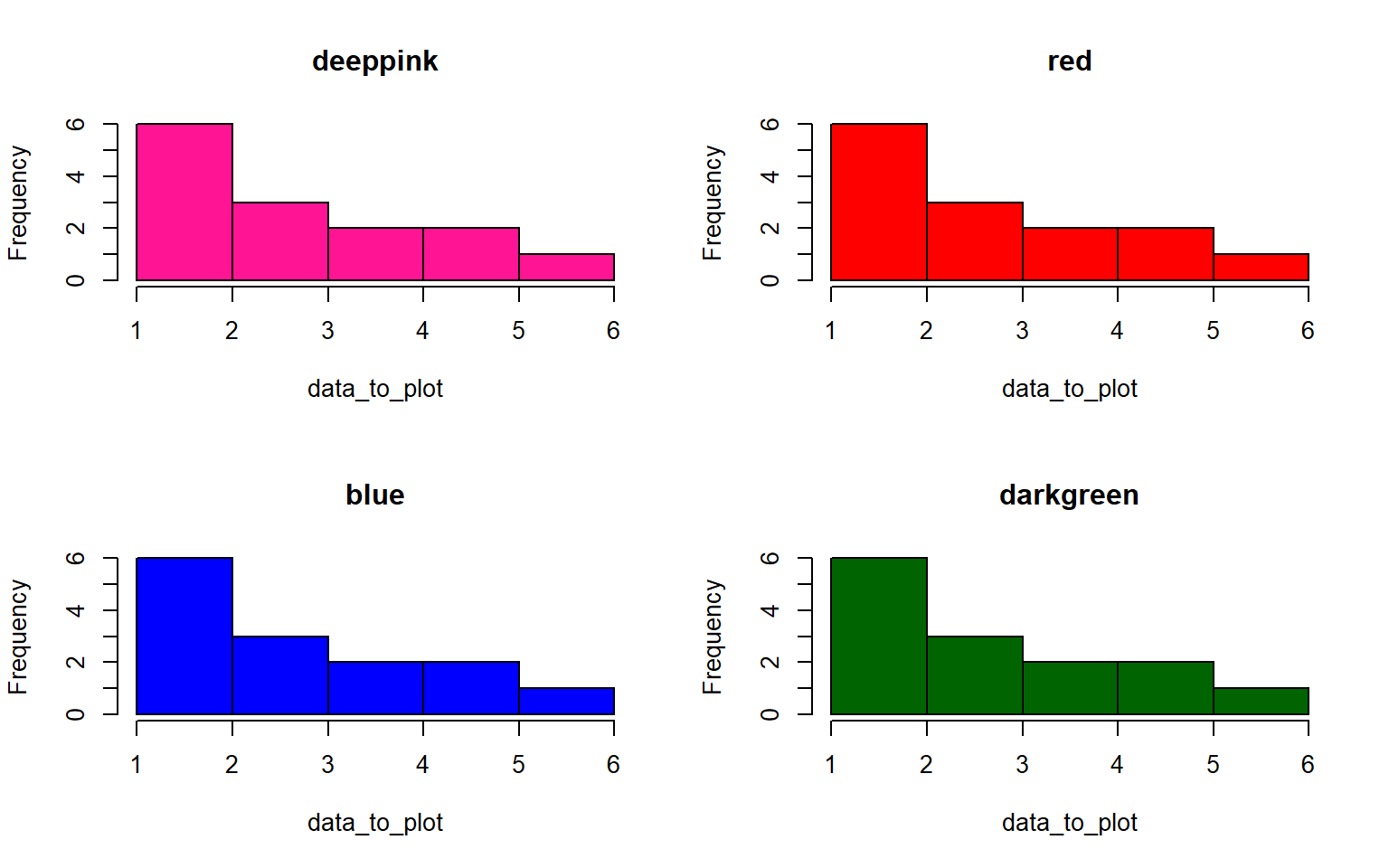
#>          deeppink       red            blue           darkgreen
#> breaks   integer,6      integer,6      integer,6      integer,6
#> counts   integer,5      integer,5      integer,5      integer,5
#> density  numeric,5      numeric,5      numeric,5      numeric,5
#> mids     numeric,5      numeric,5      numeric,5      numeric,5
#> xname    "data_to_plot" "data_to_plot" "data_to_plot" "data_to_plot"
#> equidist TRUE           TRUE           TRUE           TRUE
- Standardize all the variables in the states dataset and save your answer to a new dataframe, states_standardized Hint: to standardize a variable, you subtract the mean and divide by the standard deviation (sd)
Solution
states_standardized = apply(states, 2, function(x) (x-mean(x))/sd(x))
# original:
head(states)
#>            Population Income Illiteracy Life Exp Murder HS Grad Frost   Area
#> Alabama          3615   3624        2.1    69.05   15.1    41.3    20  50708
#> Alaska            365   6315        1.5    69.31   11.3    66.7   152 566432
#> Arizona          2212   4530        1.8    70.55    7.8    58.1    15 113417
#> Arkansas         2110   3378        1.9    70.66   10.1    39.9    65  51945
#> California      21198   5114        1.1    71.71   10.3    62.6    20 156361
#> Colorado         2541   4884        0.7    72.06    6.8    63.9   166 103766
# standardized
head(states_standardized)
#>            Population     Income Illiteracy   Life Exp     Murder    HS Grad      Frost       Area
#> Alabama    -0.1414316 -1.3211387   1.525758 -1.3621937  2.0918101 -1.4619293 -1.6248292 -0.2347183
#> Alaska     -0.8693980  3.0582456   0.541398 -1.1685098  1.0624293  1.6828035  0.9145676  5.8093497
#> Arizona    -0.4556891  0.1533029   1.033578 -0.2447866  0.1143154  0.6180514 -1.7210185  0.5002047
#> Arkansas   -0.4785360 -1.7214837   1.197638 -0.1628435  0.7373617 -1.6352611 -0.7591257 -0.2202212
#> California  3.7969790  1.1037155  -0.114842  0.6193415  0.7915396  1.1751891 -1.6248292  1.0034903
#> Colorado   -0.3819965  0.7294092  -0.771082  0.8800698 -0.1565742  1.3361400  1.1838976  0.3870991
- Create a histogram again for each variable in the states data, but this time label each histogram with the variable names when you plot Hint: instead of using apply to iterate over the columns themselves, you can often iterate over the column names with sapply
Solution
par(mfrow = c(2,2))
sapply(colnames(states), function(x)hist(states[ , x],main = x, xlab = x,col = "darkblue"))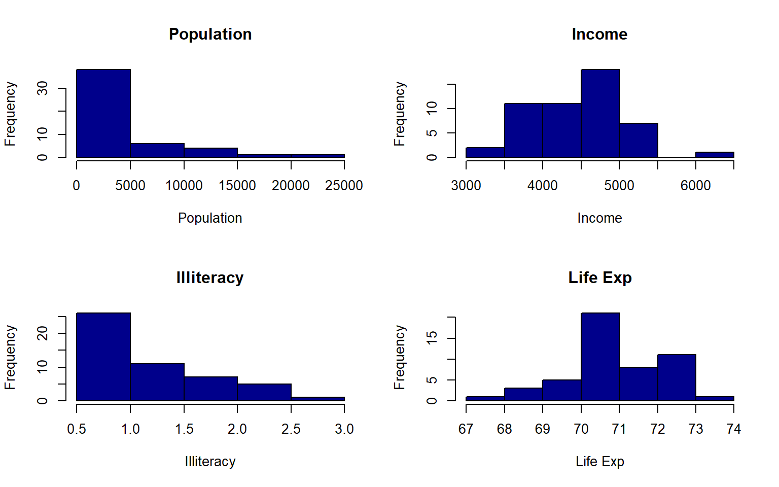
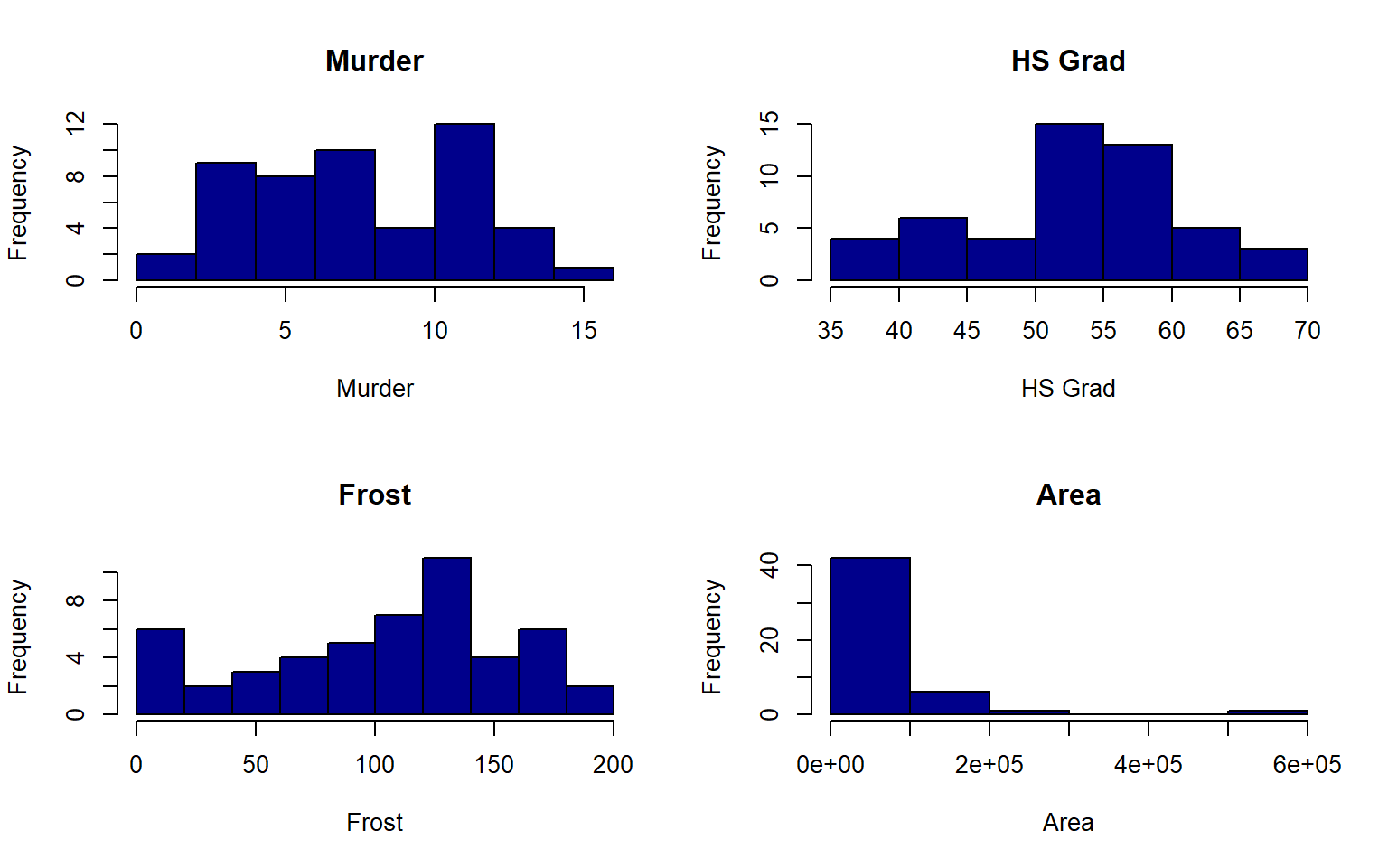
#>          Population    Income        Illiteracy    Life Exp      Murder        HS Grad       Frost         Area
#> breaks   numeric,6     integer,8     numeric,6     integer,8     numeric,9     integer,8     numeric,11    numeric,7
#> counts   integer,5     integer,7     integer,5     integer,7     integer,8     integer,7     integer,10    integer,6
#> density  numeric,5     numeric,7     numeric,5     numeric,7     numeric,8     numeric,7     numeric,10    numeric,6
#> mids     numeric,5     numeric,7     numeric,5     numeric,7     numeric,8     numeric,7     numeric,10    numeric,6
#> xname    "states[, x]" "states[, x]" "states[, x]" "states[, x]" "states[, x]" "states[, x]" "states[, x]" "states[, x]"
#> equidist TRUE          TRUE          TRUE          TRUE          TRUE          TRUE          TRUE          TRUE
For the final day covering basics in R we will have a coding session where we tackle a challenge exercise on a dataset.
Please download the exercise here
wget https://raw.githubusercontent.com/BayLab/MarineGenomicsData/main/R_Final_Challenges/chickWeightChallenge_week7_semester.RAnd the solutions are here
wget https://raw.githubusercontent.com/BayLab/MarineGenomicsData/main/R_Final_Challenges/ChickWeight_Challenge_SOLUTIONS.pdf